
How to Build a Trading Algorithm: Step-by-Step Guide

The fastest reliable path to a working trading algorithm is a disciplined workflow: define a testable hypothesis, secure clean historical data, design simple entry and exit rules, backtest rigorously, validate out-of-sample, paper trade for a couple of months, then deploy with active monitoring. That sequence works whether you write every line yourself or use a no-code platform.
Two quick recommendations before you go further. If you code, start with a minimal Python strategy using a library like pandas or NumPy and institutional-quality OHLC data. If you prefer no-code, use a deterministic platform that guarantees reproducible backtests, so you skip the plumbing and move straight to validation. Quantgenie is built exactly for that second path. On the regulatory side, the SEC and FINRA both require that automated strategies comply with existing market conduct rules, so document your logic from day one. Most strategies that look great in backtests fail live, largely because of look-ahead bias and overfitting — which is exactly why the validation steps in this guide are non-negotiable.
Table of Contents
- Which path should you take to build a trading algorithm?
- How do you build a trading algorithm from idea to live?
- What data do you need, and how do broker APIs affect your results?
- How do you backtest properly and avoid common mistakes?
- How do you go from paper trading to live deployment?
- What tools do you need to build and run a trading algorithm?
- A minimal moving-average crossover strategy, two ways
- Why do deterministic builds matter for reliable trading algorithms?
- Key Takeaways
- The mistake that costs most beginners six months
- Quantgenie gets you to validated deployment faster
- Useful sources for further reading
Which path should you take to build a trading algorithm?
There are two genuinely different ways to approach algorithmic trading development, and picking the wrong one costs weeks.
Code-first means writing your strategy in Python (or occasionally R or C++), wiring up your own data pipeline, and running backtests through a framework you control. You get maximum flexibility: custom signals, exotic instruments, proprietary data sources, and full ownership of every assumption. The tradeoff is real. You spend significant time debugging data ingestion, timestamp alignment, and execution simulation before you ever test a single trade idea. Expect days to weeks just to get a clean backtesting environment running.
No-code deterministic builders let you describe rules in plain English or drag-and-drop logic blocks, then generate a validated algorithm automatically. The key word is deterministic: the same inputs always produce the same output, which means your backtest is auditable and reproducible. Speed to validated deployment is the main advantage. You can go from idea to a complete backtest report in hours rather than days.
Who each path actually fits
Code-first suits traders who already know Python, want to model complex multi-leg strategies, or plan to integrate proprietary data feeds. Budget at least 10–20 hours per week and expect a learning curve on data quality alone. Capital thresholds matter less here than time and technical patience.
No-code builders suit traders who have a clear market thesis but limited programming background, or experienced traders who want to test ideas quickly without rebuilding infrastructure. The tradeoff is less raw customization, though modern deterministic platforms cover the vast majority of retail and professional strategy types.
When to pick each path
- Pick code-first if you need custom signals, unusual instruments, or plan to run high-frequency strategies where microsecond-level control matters.
- Pick no-code if your priority is speed to a validated, reproducible backtest and you want broker integration without writing API wrappers.
- Pick no-code if you are new to algorithmic trading and want to learn strategy logic before getting buried in infrastructure.
- Pick code-first if you want to contribute to or build on open-source frameworks like Freqtrade for crypto or similar community ecosystems.
| Dimension | Entry-level scripting tools | Deterministic no-code builders | Enterprise platforms |
|---|---|---|---|
| Reproducibility | Manual discipline required | Built-in by design | Varies by vendor |
| Data quality | User-sourced | Institutional-grade (platform-provided) | Premium, often proprietary |
| Backtesting rigor | Framework-dependent | Walk-forward and out-of-sample included | Full suite, high cost |
| Broker integrations | API coding required | Pre-built connectors | Extensive, managed |
| Ease of use | Moderate to high technical skill | Minimal technical skill | High skill or vendor support |
| Pricing | Low to free (data costs extra) | Subscription-based | Enterprise contracts |
How do you build a trading algorithm from idea to live?
The workflow below applies to both paths. What changes is the tooling, not the sequence.
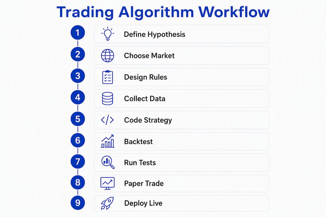
Step 1: Define your hypothesis
Write one sentence describing the market inefficiency you believe exists. “Large-cap equities tend to revert to their 20-day moving average after a 3% single-day decline” is a hypothesis. “I think stocks go up” is not. A testable hypothesis is the foundation of every durable algorithm — without it, you are fitting noise.
Step 2: Choose your market and timeframe
Pick one instrument and one timeframe to start. U.S. equities on daily bars are the most accessible for beginners: data is clean, corporate action adjustments are well-documented, and broker APIs are mature. Intraday strategies on futures or forex introduce latency and data complexity that beginners routinely underestimate.
Step 3: Design entry, exit, and position sizing rules
Keep it to 2–4 rules total. Entry: the signal that triggers a trade. Exit: both a profit target and a stop-loss. Position sizing: how much capital per trade, typically a fixed percentage of equity (1–2% risk per trade is a common starting point). Define exits as precisely as entries — vague exits produce optimistic backtests that collapse in live trading.

Step 4: Collect and clean your data
You need adjusted OHLCV data (open, high, low, close, volume) with corporate action corrections. Missing bars, duplicate timestamps, and unadjusted splits will silently corrupt your backtest. Validate your data before writing a single rule.
Step 5: Code or configure your strategy
For Python, implement your signal logic, then wrap it in a backtesting loop that processes bars sequentially — never peeking at future data. For no-code, map your rules to the platform’s input fields and confirm the parameter settings match your hypothesis exactly.
Step 6: Backtest in-sample, then out-of-sample
Split your data: roughly 70% for development (in-sample) and 30% held out for validation (out-of-sample). Never optimize parameters on the full dataset. The out-of-sample result is the only number that tells you something real.
Step 7: Run robustness tests
Walk-forward analysis and Monte Carlo simulation are the two tests that separate durable strategies from curve-fit ones. Walk-forward rolls your optimization window forward in time. Monte Carlo randomizes trade order and entry timing to stress-test drawdown scenarios.
Step 8: Paper trade for 30–60 days
Paper trading for 30–60 days reveals execution issues — slippage, order fill delays, and live-data interruptions — that backtests cannot replicate. Log every fill and compare it against your backtest assumptions. If the gap is large, revisit your cost model before going live.

Step 9: Deploy at small scale, then monitor
Start with small position sizes below your intended target. Monitor fills, latency, and equity curve daily for an initial period. Only scale up after the live results track your paper-trade period within a reasonable margin.
Timeline and cost expectations
| Setup type | Time to first live trade | Typical monthly cost |
|---|---|---|
| Hobbyist (Python, free data) | 4 weeks | $0–$50 (brokerage fees only) |
| Serious retail (paid data, no-code platform) | 2–6 weeks | $50 |
| Small professional (multi-asset, managed infra) | 8–20 weeks | $1,500+ |
Before you write a single line of code or configure a single rule, confirm you have: basic trading knowledge, starting capital you can afford to lose, a reliable computer and internet connection, a brokerage account that supports automated execution, and a documented time commitment. These five preconditions are not optional — skipping any one of them creates problems that surface at the worst possible moment.
What data do you need, and how do broker APIs affect your results?
Data quality is where most beginner algorithms quietly fail. The backtest looks fine; the live results don’t. The gap is almost always in the data.
Data types and when they matter
End-of-day OHLCV is sufficient for daily swing strategies and is the easiest to source cleanly. Intraday OHLCV (1-minute, 5-minute bars) is needed for strategies that trade within a session — and the data volume and cleaning burden multiply fast. Tick data is necessary for high-frequency strategies and is expensive to store and process. Corporate action adjustments (splits, dividends) are non-negotiable for equity strategies: unadjusted data produces phantom signals around split dates. Alternative data — volume profiles, news sentiment, options flow — adds complexity and is rarely worth it until your baseline strategy is validated.
Common data quality pitfalls
Survivorship bias is the most dangerous and least obvious. If your historical dataset only includes companies that still exist today, your backtest is testing on a universe of survivors and will overstate performance. Use a point-in-time dataset that includes delisted securities. Missing bars, duplicate rows, and timezone mismatches are mechanical issues that a data validation script catches before they corrupt results.
Broker API considerations
Not all broker APIs are equal for algorithmic trading. Key factors: supported order types (market, limit, stop, bracket), fractional share availability, paper-trading sandbox quality, rate limits per second, and WebSocket vs REST latency. Interactive Brokers’ TWS API is one of the most widely used for U.S. equities and futures, with mature Python client libraries. Alpaca offers a REST API with paper-trading support that suits beginners well. TD Ameritrade’s thinkorswim platform has its own scripting environment for retail traders.
Latency matters differently depending on strategy frequency. A daily swing strategy can tolerate seconds of latency. An intraday mean-reversion strategy cannot. Know your frequency before choosing a broker.
Pro Tip: Model slippage and commissions explicitly in every backtest. A strategy that earns 0.3% per trade before costs often earns nothing after a realistic $0.005-per-share commission and one-tick slippage assumption. If your edge disappears when you add realistic costs, it was never an edge.
How do you backtest properly and avoid common mistakes?
Backtesting is necessary but not sufficient. Strategies that backtest well frequently fail live because of look-ahead bias and overfitting. The backtest is a hypothesis test, not a performance guarantee.
The validation checklist
- Use clean, adjusted, point-in-time data with no survivorship bias.
- Align timestamps precisely — bar close must not include data from the next bar.
- Include realistic transaction costs: commissions, slippage, and spread.
- Split data into in-sample (development), validation, and out-of-sample (test) sets — never optimize on the test set.
- Run walk-forward analysis and Monte Carlo simulations to stress-test drawdown and parameter sensitivity.
- Require a minimum trade count before trusting any metric — fewer than 30–50 trades produces statistically meaningless results.
- Test across multiple market regimes: bull, bear, and sideways conditions each expose different failure modes.
Pitfalls that kill otherwise good strategies
Look-ahead bias is using future data to generate a past signal — the most common coding error in backtesting. It produces spectacular results that vanish immediately in live trading. Survivorship bias inflates returns by excluding failed securities. Curve-fitting (also called HARKing — Hypothesizing After Results are Known) means adding parameters until the backtest looks good, rather than testing a pre-specified hypothesis. Parameter snooping is running hundreds of parameter combinations and reporting only the best one without adjusting for multiple comparisons.
The warning sign for all of these is the same: unusually strong early metrics. A Sharpe ratio above 3.0 on in-sample data, a profit factor above 4.0, or a maximum drawdown below 5% on a daily equity strategy should trigger skepticism, not celebration. Excessive early high metrics often indicate overfitting, not a genuine edge.
Metrics that matter
Track profit factor (gross profit divided by gross loss), Sharpe ratio, maximum drawdown, and average trade duration. A profit factor above 1.3 with a Sharpe above 1.0 and a drawdown you can psychologically tolerate is a reasonable baseline. These numbers mean nothing without the trade count to support them.
How do you go from paper trading to live deployment?
Deployment is where the algorithm meets reality, and reality is messier than any backtest.
Paper trading best practices
Run your algorithm in a paper-trading environment for a full 30–60 days with real-time data, not simulated fills. Log every order: intended entry price, actual fill price, slippage, and timestamp. Compare the paper-trade equity curve against your backtest projections weekly. If the paper results diverge significantly, stop and diagnose before going live.
Deployment checklist
- Confirm broker credentials, API permissions, and order type support before the first live order.
- Implement execution error handling: what happens if an order is rejected, partially filled, or times out?
- Set circuit breakers: a maximum daily loss limit that halts the algorithm automatically.
- Define position limits: maximum exposure per instrument and total portfolio exposure.
- Build an automated risk shutdown: if drawdown exceeds a pre-set threshold (e.g., 10% from peak), the algorithm stops and alerts you.
- Store all logs: order history, fill confirmations, and error messages.
Monitoring metrics to track daily
- Fills vs. expected fills (slippage tracking)
- Order latency from signal to execution
- Equity curve vs. paper-trade baseline
- Current drawdown from peak
- Per-trade slippage vs. backtest assumption
Incident response
Set automated alerts for anomalies: unexpected position sizes, order rejections above a threshold, or equity drops beyond a daily limit. Have a manual override procedure documented before you go live — not after something goes wrong. After any unexpected behavior, run a post-mortem: pull the logs, identify the root cause, and update your error-handling code before restarting.
What tools do you need to build and run a trading algorithm?
The right toolset depends on your path, but certain features are non-negotiable regardless of approach.
Features to prioritize in any tool or platform
- Deterministic reproducible builds: the same inputs must always produce the same backtest output. Without this, you cannot audit your results or compare runs reliably.
- Quality historical data: adjusted, point-in-time, exchange-level price data with corporate actions handled correctly.
- Walk-forward and out-of-sample backtesting: not just a simple equity curve, but structured validation across time periods.
- Broker integrations: pre-built or well-documented connections to U.S. brokers for paper and live execution.
- Logging and alerting: production-grade monitoring so you know immediately when something breaks.
- Documentation and support: especially important for beginners who hit unexpected edge cases.
Tool categories for the code-first path
Python is the dominant language for retail algorithmic trading. The core libraries are pandas for data manipulation, NumPy for numerical computation, and Matplotlib or Plotly for visualization. For backtesting frameworks, QuantConnect offers a cloud-based environment with multi-asset support and realistic cost modeling. Interactive Brokers provides Python-based backtesting and execution tutorials that are worth studying for their modular architecture. Freqtrade handles crypto-specific backtesting with built-in optimization and Telegram-based monitoring.
For data, Quandl (now part of Nasdaq Data Link), Polygon.io, and Alpha Vantage cover most retail needs for U.S. equities. For futures and forex, CME Group’s data services and OANDA’s API are standard starting points.
The no-code path: what to look for
A no-code platform earns its subscription fee only if it delivers three things: deterministic algorithm generation, institutional-grade historical data, and transparent backtest metrics. Quantgenie delivers all three. You describe your strategy in plain English or use the visual builder, and the platform translates it into a deterministic algorithm with reproducible runs. Every backtest produces the same output under the same conditions, which means you can audit, compare, and iterate without worrying that a result changed because of a hidden random seed or data-loading quirk. For traders who want to reach validated deployment faster without sacrificing rigor, that is the practical advantage.
A minimal moving-average crossover strategy, two ways
The moving-average crossover is the standard starting point for a reason: it is simple, transparent, and tests cleanly across market regimes.
Hypothesis: When a short-term moving average crosses above a long-term moving average, the instrument is in an uptrend and a long position is warranted. Exit when the short crosses back below the long.
Rules:
- Market: U.S. large-cap equity (e.g., SPY ETF)
- Timeframe: Daily bars
- Entry: Buy at next open when 10-day SMA crosses above 50-day SMA
- Exit: Sell at next open when 10-day SMA crosses below 50-day SMA
- Position size: 100% of capital (single-position, for simplicity)
- Stop: No hard stop (exit rule handles it)
Python implementation (minimal)
import pandas as pd

# Load adjusted daily OHLCV — replace with your data source
df = pd.read_csv("SPY_daily_adjusted.csv", parse_dates=["Date"], index_col="Date")
df = df.sort_index()

# Split: first 70% in-sample, last 30% out-of-sample
split = int(len(df) * 0.7)
train = df.iloc[:split].copy()
test  = df.iloc[split:].copy()

def run_backtest(data):
    data = data.copy()
    data["SMA10"] = data["Close"].rolling(10).mean()
    data["SMA50"] = data["Close"].rolling(50).mean()
    data["Signal"] = 0
    data.loc[data["SMA10"] > data["SMA50"], "Signal"] = 1
    data["Position"] = data["Signal"].shift(1)          # enter at next open
    data["Return"]   = data["Close"].pct_change()
    data["Strategy"] = data["Position"] * data["Return"]
    cumulative = (1 + data["Strategy"]).cumprod()
    sharpe = (data["Strategy"].mean() / data["Strategy"].std()) * (252 ** 0.5)
    max_dd = (cumulative / cumulative.cummax() - 1).min()
    return {"Sharpe": round(sharpe, 2), "Max Drawdown": round(max_dd, 2),
            "Total Trades": int(data["Position"].diff().abs().sum() // 2)}

print("In-sample: ", run_backtest(train))
print("Out-of-sample:", run_backtest(test))
This snippet is intentionally minimal. It does not model commissions or slippage — add those before drawing any conclusions. The shift(1) on the signal is what prevents look-ahead bias: you only act on yesterday’s signal at today’s open.
No-code equivalent in a deterministic builder
- Open Quantgenie’s visual strategy builder and create a new strategy.
- Set the instrument to SPY and the timeframe to Daily.
- Add Entry Rule: “10-day simple moving average crosses above 50-day simple moving average.”
- Add Exit Rule: “10-day simple moving average crosses below 50-day simple moving average.”
- Set position sizing to a fixed percentage of portfolio equity.
- Configure the data split: 70% in-sample, 30% out-of-sample.
- Run the backtest. The platform generates a deterministic result log — the same parameters will produce the same output on every run.
- Review the generated report: Sharpe ratio, profit factor, maximum drawdown, number of trades, and the out-of-sample equity curve.
- If out-of-sample metrics are materially weaker than in-sample, the strategy is likely overfit. Simplify before paper trading.
Timeline: Python path takes 4–8 hours to get a clean, reproducible result for a beginner. The no-code path in Quantgenie takes 30–60 minutes for the same strategy, with the validation report generated automatically.
| Step | Python path | No-code path (Quantgenie) |
|---|---|---|
| Data setup | 1–3 hours | Included in platform |
| Signal coding / configuration | 1–2 hours | 30 minutes |
| Backtest and validation | 1–2 hours | Automated |
| Out-of-sample report | Manual calculation | Auto-generated |
| Total time (beginner) | 4–8 hours | 30–60 minutes |
Why do deterministic builds matter for reliable trading algorithms?
Most traders focus on the strategy. The platform’s architecture is what actually determines whether your backtest means anything.
A non-deterministic backtest is one where re-running the same strategy with the same parameters produces a slightly different result. That happens when platforms use random seeds for simulation, inconsistent data loading, or floating-point operations that vary by run. The practical consequence: you cannot tell whether a change in performance came from a rule adjustment or from platform noise. Auditing becomes impossible.
Quantgenie’s deterministic generation means every run is identical under identical conditions. That matters for three reasons. First, you can compare strategy versions with confidence — any performance difference is real. Second, you can share a strategy configuration and have someone else reproduce your exact results. Third, for traders operating under any form of oversight or compliance review, reproducible audit logs are not optional.
Trust signals to look for in any platform
- Reproducible run logs: every backtest stores the exact parameters, data version, and output metrics.
- Out-of-sample metrics reported separately: not blended with in-sample results.
- Walk-forward reports: showing performance across rolling time windows, not just a single historical period.
- Documented data provenance: which exchange, which adjustment method, which date range.
- AI-assisted result interpretation: Quantgenie’s built-in question-answering lets you interrogate your backtest results in plain English, which is particularly useful when a metric looks unexpected.
What to request or verify before trusting a platform’s backtest
- Can you re-run the identical backtest and get the identical output?
- Does the platform disclose its data source and adjustment methodology?
- Are walk-forward and out-of-sample tests built in, or do you have to implement them manually?
- Does the platform model commissions and slippage, or does it report gross returns?
- Is there a paper-trading mode connected to real broker infrastructure?
Quantgenie checks all of these. For traders who want institutional-grade validation without building the infrastructure themselves, that combination is the practical argument for the platform.
Key Takeaways
Building a trading algorithm requires a disciplined workflow, clean data, robust validation, and continuous monitoring — no shortcut in that sequence produces reliable live results.
| Point | Details |
|---|---|
| Start with a testable hypothesis | Write one sentence describing the market inefficiency before touching any code or platform. |
| Validate beyond the backtest | Run walk-forward analysis and out-of-sample tests; in-sample performance alone is not evidence of a real edge. |
| Paper trade for 30–60 days | An effective paper trading period is 30–60 days, which reveals slippage and fill issues that backtests cannot replicate. |
| Keep rules simple | Limit your strategy to 2–4 rules; more parameters increase overfitting risk, not performance. |
| Use Quantgenie for reproducible builds | Quantgenie translates plain-English rules into deterministic algorithms with institutional-grade backtesting and broker integration. |
The mistake that costs most beginners six months
The most common early mistake in algorithmic trading development is not a coding error. It is adding parameters.
A strategy underperforms in the backtest, so you add a filter. Then another. Then a volatility regime condition. Then a time-of-day exclusion. Each addition improves the in-sample result, and each one makes the strategy more fragile out-of-sample. By the time you deploy, you have a strategy that fits the past perfectly and predicts the future no better than chance.
The fix is uncomfortable: go back to 2–4 rules and accept that a simpler strategy with a modest edge is worth more than a complex one with a spectacular backtest. Industry practitioners consistently find that the most successful algorithms are simple and transparent — traders who can explain the market logic behind every trade are the ones who survive regime shifts.
One practical habit that separates serious builders from hobbyists: maintain a changelog. Every time you change a parameter, add a rule, or switch a data source, log the date, the reason, and the before/after metrics. Version-control your strategy files the same way a software engineer versions code. Then run a scheduled robustness test after every change — not just when you feel like it. Strategies that looked solid in January can degrade quietly by June as market conditions shift, and a monthly walk-forward check catches that before it costs real capital.
The other thing beginners consistently underestimate is the operational gap between building an algorithm and running one. Maintaining a live trading system requires separate skills from building it: monitoring, risk management, incident response, and periodic revalidation after regime shifts are ongoing processes, not one-time tasks. Budget time for operations, not just development.
Quantgenie gets you to validated deployment faster
If the workflow in this guide sounds like a lot of infrastructure to build before you test a single idea, that is because it is. The code-first path is powerful, but the setup cost is real.
Quantgenie removes that friction without removing the rigor. You describe your strategy in plain English or use the visual builder, and the platform generates a deterministic algorithm with institutional-grade historical data already wired in. Backtests are reproducible by design — re-run the same strategy and get the same result, every time. Walk-forward analysis and out-of-sample validation are built into the workflow, not optional add-ons. When you are ready to trade, direct broker integrations handle paper and live execution without you writing a single API wrapper.
The practical result: a trader who would spend 4–8 hours getting a clean Python backtest running can get a validated, reproducible result in under an hour on Quantgenie. That time difference compounds across every strategy iteration.
Start building on Quantgenie and run your first deterministic backtest today. When you do, apply the validation checklist from this guide — even on a no-code platform, the discipline of out-of-sample testing and paper trading is what separates a strategy worth deploying from one that just looks good on paper.
Useful sources for further reading
- How to Code Your Own Algo Trading Robot (Investopedia) — practical overview of look-ahead bias, overfitting risks, and the case for out-of-sample validation.
- Basic Trading Algorithms in Python (IBKR Quant) — hands-on Python tutorial using pandas and NumPy with Interactive Brokers’ execution infrastructure.
- Build a Custom Backtester with Python (IBKR Quant) — modular backtester architecture guide; useful for code-first traders who want a maintainable, extensible framework.
- Freqtrade on GitHub — open-source crypto trading bot with built-in backtesting, walk-forward optimization, and Telegram-based monitoring; a practical reference for the code-first path.
- Algorithmic Trading Courses (Coursera) — structured learning paths for traders who want to build foundational knowledge before writing production code.