
Monte Carlo Backtesting for Traders: Robustness Checks

Monte Carlo backtesting converts your single historical equity curve into a distribution of many plausible alternate trade histories, so you can measure how much of your observed edge was structural versus lucky sequencing. The immediate next step: run a reshuffle (trade-order randomization) with a practical minimum of iterations, record drawdown percentiles such as P5 and P50, and pair it with an in-sample/out-of-sample split. Before trusting any Monte Carlo output, apply this overfitting veto rule: if out-of-sample Sharpe drops significantly or win-rate gap exceeds a small margin versus in-sample, disqualify the strategy regardless of how good the percentiles look.
- Core claim: One backtest is one path. Monte Carlo shows you the distribution of paths your trade sequence could have produced.
- Immediate action: Run a 1,000-iteration reshuffle, log your seed, and record P5, P50, and worst-case max drawdown.
- Veto rule: Out-of-sample Sharpe drop >0.5 or win-rate gap >5pp disqualifies the strategy, full stop.
Table of Contents
- What is Monte Carlo backtesting, and what are the main variants?
- Why should you run Monte Carlo on your backtests?
- How do the four Monte Carlo methods compare in practice?
- How do you run a Monte Carlo backtest step by step?
- How do you read Monte Carlo output and translate it into decisions?
- What are the real limitations of Monte Carlo, and how do you work around them?
- Why combining two Monte Carlo categories gives you a fuller picture
- Which tools should you use for Monte Carlo backtesting?
- What should a Monte Carlo robustness report include?
- Key Takeaways
- Why most traders use Monte Carlo wrong
- Quantgenie makes reproducible robustness checks accessible
- Useful sources and further reading
What is Monte Carlo backtesting, and what are the main variants?
Monte Carlo backtesting re-samples or perturbs the realized backtest, whether that means shuffling trade order, resampling trades with replacement, or altering the underlying price data, to produce many plausible equity curves and a distribution of performance metrics. The realized backtest is just one path through a much larger space of possible outcomes. Monte Carlo maps that space.
There are four primary variants, each answering a different robustness question:
- Trade-order reshuffle: Randomizes the sequence of realized trades while keeping each trade’s return intact. Best for measuring path-dependence and drawdown risk, since the same trades in a different order can produce wildly different max drawdowns.
- Bootstrap/resample: Draws trades with replacement from the realized set, allowing the same bad trade to appear multiple times. This widens the distribution and produces more pessimistic tails than reshuffle, because unlucky draws can stack repeated losses.
- Candle/price perturbation: Alters the price series itself, either by adding noise or using block-bootstrap on candles to preserve serial correlation. Useful when intraday structure or autocorrelation matters to the strategy’s execution.
- Parameter perturbation: Jitters rule parameters by ±x% to expose curve-fit brittleness. A strategy with genuine edge degrades gracefully under small parameter shifts; an overfit one collapses.
The two-category taxonomy practitioners recommend most is trade-order shuffling combined with parameter or data perturbation. Together they test both path-dependence and structural robustness, which no single method covers alone.
Why should you run Monte Carlo on your backtests?
A single backtest tells you what happened on one specific path through history. It says nothing about whether a different ordering of those same trades would have blown up your account, or whether your Sharpe ratio depends on three lucky months in 2021. Monte Carlo answers both questions.
The primary benefits break down into three categories:
- Drawdown quantification: Instead of one max drawdown figure, you get a distribution. The P5 drawdown tells you what to expect in the worst 5% of plausible histories, which is the number that should drive your position sizing and kill-switch thresholds.
- Path-dependence exposure: Some strategies look fine on average but have catastrophic sequences. Reshuffle Monte Carlo surfaces these without requiring new historical data.
- Sizing and live-readiness inputs: Percentile-based risk numbers give you a principled basis for deciding how much capital to risk per trade and whether to deploy at all.
Monte Carlo replaces single-point estimates with probability distributions that support percentile-based decision-making, specifically P50 for median expectation, P75/P90 for contingency reserves, and P5/P10 for downside stress.
Iteration guidance: 1,000 iterations is the practical minimum for standard checks. Use 5,000–10,000 when tail stability matters. For P99 or probability-of-ruin analysis, 50,000–100,000 iterations may be necessary.
Monte Carlo also helps you prioritize model improvements. If reshuffle keeps P5 positive but parameter perturbation collapses it, the structural logic is fragile, not the sequencing. That tells you exactly where to focus.
How do the four Monte Carlo methods compare in practice?

Each method tests a different assumption about where your strategy’s fragility lives. Choosing the right one, or the right combination, depends on what question you are actually trying to answer.
| Method | What it tests | Key assumption | Typical iteration range |
|---|---|---|---|
| Trade-order reshuffle | Path-dependence, drawdown sensitivity | Trade returns are independent | 1,000–5,000 |
| Bootstrap/resample | Sampling uncertainty, tail risk | Trades are exchangeable | 1,000–5,000 |
| Candle/price perturbation | Price-level sensitivity, execution friction | Serial correlation preserved via block-bootstrap | 1,000–10,000 |
| Parameter perturbation | Curve-fit brittleness | Small parameter shifts should not collapse performance | 1,000–5,000 |
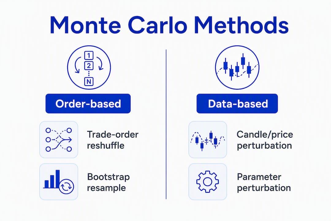
Reshuffle is the fastest and most intuitive starting point. It preserves every trade’s return but randomizes the sequence, so the only thing changing is the order in which gains and losses arrive. Max drawdown is highly sensitive to this, which is exactly why reshuffle is the right tool for path-dependent metrics.
Bootstrap/resample goes further by allowing bad trades to repeat. Because it draws with replacement, the tails are wider and more pessimistic than reshuffle. Use it when you want a conservative estimate of sampling uncertainty, particularly when your trade sample is small.
Candle/price perturbation is the method most traders skip, and often the one that matters most for intraday strategies. Naive reshuffle breaks serial correlation in price data, which can produce misleadingly optimistic results for strategies that depend on momentum or mean-reversion persistence. Block-bootstrap or candle-level perturbation preserves that structure.

Parameter perturbation is the sharpest test of curve-fit. Jitter your entry threshold, lookback period, or stop-loss level by a few percent in each direction. If performance degrades smoothly, the edge is real. If it falls off a cliff at ±2%, you have a curve-fit problem that no amount of reshuffle analysis will fix.
Pro Tip: Run parameter perturbation last, after reshuffle and bootstrap have confirmed path-independence. A strategy that passes reshuffle but fails parameter perturbation is structurally fragile, and that failure is a stronger disqualifier than a poor P5 on reshuffle alone.
For correlated strategies, always use block-bootstrap rather than naive reshuffle. Preserving block lengths keeps the autocorrelation structure intact and prevents the simulation from generating unrealistic trade sequences.
How do you run a Monte Carlo backtest step by step?
The workflow is the same whether you are working in Excel, Python, or a platform. What changes is the speed, reproducibility, and depth of logging.
Prepare your inputs first. Export trade-level P&L with timestamps, position sizes, and your baseline slippage and commission assumptions. Confirm the data window is consistent — mixing regimes without documentation is one of the most common sources of misleading Monte Carlo results. Apply a clean in-sample/out-of-sample split before you run a single simulation.
Then follow these steps:
- Lock your seed and baseline assumptions. Set a fixed random seed (e.g.,
numpy.random.seed(42)in Python) and document slippage, commission, and position-sizing rules. Without a fixed seed, your results are not reproducible. - Choose your method and iteration count. Start with reshuffle at 1,000 iterations for a quick check. Move to 5,000–10,000 if you need stable tail estimates. Add bootstrap and parameter perturbation as a second pass.
- Run n iterations and collect metrics. For each iteration, record terminal portfolio value, max drawdown, Sharpe ratio, and win rate. Store the full distribution, not just summary statistics.
- Compute percentiles and drawdown histories. Calculate P5, P50, and P95 terminal values. Build the max drawdown distribution. Identify where the realized backtest sits within the simulated distribution.
- Apply the in-sample/out-of-sample veto. If the out-of-sample Sharpe drops more than 0.5 or win-rate gap exceeds 5 percentage points, disqualify the strategy. Monte Carlo percentiles do not override this check.
Checklist before you finalize:
- Minimum 30 trades in the sample for meaningful statistics (fewer trades produce unstable percentiles)
- Seed and RNG type documented
- Slippage and commission assumptions written down, not assumed
- Code snapshot or export saved alongside results
- In-sample/out-of-sample split applied and recorded
The minimum-trade rule deserves emphasis. With 15 trades, your P5 estimate is essentially one data point. With 100 trades, the distribution stabilizes enough to trust.
How do you read Monte Carlo output and translate it into decisions?
The output of a Monte Carlo run is a distribution of equity curves and a set of percentile metrics. Reading it correctly is what separates traders who use Monte Carlo as a real decision tool from those who use it as a rubber stamp.
What percentiles tell you:
- P5 (5th percentile): The worst outcome in 95% of simulated histories. If P5 is above your starting capital, the strategy has a conservative edge signal. If P5 is below starting capital, the strategy loses money in 5% of plausible histories, which is a meaningful risk for live deployment.
- P50 (median): Your realistic central expectation, not the best-case. Size your position and set your return expectations here, not at P95.
- P95 (95th percentile): The upside tail. Useful for understanding the ceiling, but never use it for sizing or planning.
The equity envelope check is where most traders find the most insight. Plot all simulated equity curves and overlay the realized backtest. If the realized backtest sits at or above the 90th percentile of simulated outcomes, that is a red flag. It means your actual historical path was unusually favorable, and live trading is unlikely to replicate it.
Reshuffling the sequence of realized trades shows that a realized backtest is just one path through many, and the distribution of max drawdowns across those paths is often far wider than the single realized figure suggests.
Sizing rule of thumb: Use P5/P10 drawdown figures to set your kill-switch threshold and contingency capital. Use P50 terminal value to set realistic return expectations. Never size a position based on the realized backtest’s single max drawdown figure.
Probability of ruin deserves its own calculation. Count the fraction of simulated paths that breach a defined loss threshold (say, 30% drawdown) and treat that fraction as your ruin probability. Pair this with worst-case max drawdown for psychological and capital planning. A strategy with a 2% ruin probability at 30% drawdown is a very different deployment decision than one with a 15% ruin probability at the same threshold.
What are the real limitations of Monte Carlo, and how do you work around them?
Monte Carlo is a robustness test, not a forecast. It answers one specific question: given the trades you actually made, how much did the observed performance depend on their sequence and mix? It cannot tell you whether those trades will keep occurring in the future, whether the market regime has changed, or whether your parameters are overfit to a historical window.
That distinction matters operationally. A strategy can pass Monte Carlo with flying colors and still be a curve-fit disaster if the in-sample window happened to contain a regime that no longer exists.
The most common mistakes:
- Too few iterations: Running 100 simulations gives you a noisy estimate. P5 from 100 runs is essentially the 5th-worst outcome out of 100, which is not stable.
- Ignoring serial correlation: Naive reshuffle on an intraday momentum strategy breaks the autocorrelation structure and produces unrealistically optimistic results. Use block-bootstrap when the strategy depends on price persistence.
- Anchoring on tight input ranges: If you only jitter parameters by ±1% when the realistic uncertainty is ±10%, parameter perturbation will tell you nothing useful.
- Skipping execution friction: Running Monte Carlo on gross returns and then applying slippage as an afterthought understates real drawdowns. Build slippage and commission into every iteration.
- Using Monte Carlo as a validation substitute: Monte Carlo is a robustness gate, not a green light. Always run in-sample/out-of-sample splits and walk-forward validation before or alongside it.
Practical mitigations:
- Set a minimum of 1,000 iterations for standard checks; go to 5,000+ when tails matter
- Apply block-bootstrap for any strategy with autocorrelated returns or intraday structure
- Use the in-sample/out-of-sample veto rule as a pre-filter before Monte Carlo, not an afterthought
- Document every assumption, including seed, slippage, commission, and data window, so results are reproducible and auditable
Why combining two Monte Carlo categories gives you a fuller picture
The research consensus among practitioners is that trade-order shuffling and parameter or data perturbation test fundamentally different dimensions of fragility. Using only one gives you a partial answer.
Here is what that looks like in practice. Suppose you run a reshuffle on a mean-reversion strategy. P5 stays positive across 5,000 iterations, max drawdown distribution looks acceptable, and the realized backtest sits near the median. Reshuffle passes.
Then you run parameter perturbation, jittering the lookback period and entry threshold by ±5%. Performance collapses. Sharpe drops from 1.2 to 0.3 across the parameter neighborhood. The strategy is curve-fit to a specific parameter combination, and the reshuffle result was telling you about path-dependence, not structural robustness.
The two-category approach recommended by practitioners addresses exactly this gap:
- Stage 1 (reshuffle/bootstrap): Tests ordering risk and sampling uncertainty. Confirms the edge is not purely a function of a lucky trade sequence.
- Stage 2 (parameter/data perturbation): Tests structural robustness. Confirms the edge persists across a neighborhood of parameter values and price-data variations.
Why parameter perturbation failures are stronger disqualifiers: A strategy that fails reshuffle might just have a path-dependent drawdown profile that you can manage with position sizing. A strategy that fails parameter perturbation has no stable edge to manage. The structural logic itself is fragile, and no amount of sizing adjustment fixes that.
The practical recommendation: run reshuffle first to understand ordering risk and set drawdown expectations, then run parameter perturbation to confirm the edge is not a point estimate. Treat a parameter perturbation failure as a hard stop, not a yellow flag.
Which tools should you use for Monte Carlo backtesting?
The right tool depends on your trade volume, reproducibility requirements, and how much you want to automate.
Excel is accessible and works for quick ad-hoc checks on small datasets. You can build a reshuffle simulation using RANDBETWEEN and data tables, and it is a reasonable way to learn the mechanics. The Microsoft Excel Monte Carlo approach covers the basic setup. The limitations are real, though: Excel is slow for anything above a few hundred trades and 1,000 iterations, seed control is awkward, and logging simulation configs for audit purposes is manual and error-prone. Use it for learning and ad-hoc checks, not production validation.
Python with pandas and numpy is the default for quantitative analysts. You get full seed control, parallel execution, and the ability to log every simulation config alongside results. A basic reshuffle loop runs in seconds for 1,000 iterations on a standard laptop; 10,000 iterations on a 200-trade dataset typically completes in under a minute. The reproducibility story is clean: fix numpy.random.seed, save the config as JSON, and every run is auditable.
No-code platforms are the right choice when you want repeatable, auditable runs without writing infrastructure code, or when you are working in a team where not everyone codes. The key feature to look for is exportable seeds and simulation configs. A platform that runs Monte Carlo but does not let you export the seed and method parameters is not auditable, which defeats part of the purpose.
| Tooling | Best for | Iteration ceiling (practical) | Reproducibility |
|---|---|---|---|
| Excel | Ad-hoc checks, <1,000 trades | ~1,000 | Manual, limited |
| Python (pandas/numpy) | Research and production validation | 100,000+ | Full (seed + config logging) |
| No-code platform | Team workflows, repeatable runs | Platform-dependent | High when seed export is supported |
Free Monte Carlo tools built for other domains, such as retirement planning calculators, can illustrate the mechanics but lack the trade-level inputs and seed control that strategy validation requires. They are useful for building intuition, not for production robustness checks.
For traders who want institutional-grade backtesting without building Python infrastructure, Quantgenie provides a deterministic build engine where every strategy configuration produces identical results under the same conditions. That determinism is what makes Monte Carlo scenarios auditable: you can re-run any simulation with the same seed and get the same output, which matters when you are presenting results to a risk committee or revisiting a strategy months later.
What should a Monte Carlo robustness report include?
A Monte Carlo report that a reviewer or investment committee can actually use needs two things: enough information to reproduce the results, and enough output to make a decision.
Minimum reproducibility checklist:
- Data window and universe (start date, end date, instruments, data source)
- Trade-level export (P&L, timestamps, position sizes)
- Seed and RNG type (e.g.,
numpy.random.seed(42), Mersenne Twister) - Method type: reshuffle, bootstrap, candle perturbation, parameter perturbation, or combination
- Iteration count
- Slippage and commission assumptions (per trade, per share, or percentage)
- Code snapshot or platform export (version-controlled or timestamped)
Sample output fields every report should show:
- P5, P10, P50, P95 terminal portfolio values
- Median and worst-case max drawdown
- Probability of ruin (fraction of paths breaching a defined loss threshold)
- Sample equity envelopes (a selection of simulated curves overlaid on the realized backtest)
- Sensitivity chart showing which parameters drive the most performance variance
Verdict line: Every report should close with an explicit verdict: EDGE CONFIRMED, OVERFIT, NO EDGE, or INSUFFICIENT DATA, with a one-sentence reason. “EDGE CONFIRMED: P5 positive, parameter perturbation degrades gracefully, out-of-sample Sharpe within 0.3 of in-sample” is a decision. A table of percentiles with no conclusion is not.
Key Takeaways
Monte Carlo backtesting is a robustness gate, not a forecast: combine trade-order reshuffle with parameter perturbation, apply the in-sample/out-of-sample veto, and record P5, P50, and max drawdown distribution before any live deployment decision.
| Point | Details |
|---|---|
| Run reshuffle first | Start with 1,000-iteration trade-order reshuffle; record P5, P50, and max drawdown distribution as your baseline. |
| Add parameter perturbation | A strategy that passes reshuffle but collapses under ±5% parameter jitter has no stable edge; treat this as a hard disqualifier. |
| Apply the overfitting veto | Disqualify any strategy where out-of-sample Sharpe drops >0.5 or win-rate gap exceeds 5 percentage points versus in-sample. |
| Use P5 as your sizing anchor | Size positions and set kill-switch thresholds from the P5 drawdown figure, not the single realized backtest max drawdown. |
| Quantgenie for auditable runs | Quantgenie’s deterministic build engine lets you reproduce any Monte Carlo scenario with the same seed, making results auditable and comparable across strategy iterations. |
Why most traders use Monte Carlo wrong
The conventional wisdom treats Monte Carlo as a final validation step, something you run after you have already decided a strategy is good, to confirm what you already believe. That is exactly backwards.
Monte Carlo is most useful as a filter you apply before you get attached to a strategy. Run it early, run it on strategies you expect to fail, and use the failures to calibrate what a passing result actually looks like. Most traders who run Monte Carlo for the first time are surprised by how many strategies that looked solid on a single backtest have P5 values below starting capital. That surprise is the point.
The other thing practitioners underestimate is the gap between reshuffle and parameter perturbation. Reshuffle is intuitive and the results are usually reassuring, because most strategies with a real edge survive trade-order randomization. Parameter perturbation is where the real fragility shows up, and it is the test most traders skip because it requires more setup. The strategies that fail parameter perturbation but pass reshuffle are the dangerous ones: they look robust on the metric most people check, and they fall apart on the one most people skip.
One more thing worth saying plainly: a strategy that passes every Monte Carlo test is not proven to work in live markets. It is proven to be internally consistent given the historical trade sample. Regime changes, liquidity shifts, and execution differences are not in the simulation. Monte Carlo is a necessary condition for confidence, not a sufficient one.
Quantgenie makes reproducible robustness checks accessible
Running a proper Monte Carlo workflow, with seed control, parameter perturbation, and auditable exports, typically requires either Python infrastructure or a platform built for it. Quantgenie handles the infrastructure so you can focus on the strategy.
Describe your strategy in plain English, and Quantgenie translates it into a deterministic algorithm that produces identical results every time you run it under the same conditions. That determinism is the foundation of auditable Monte Carlo testing: every simulation scenario is reproducible, every seed is logged, and every result can be compared across strategy iterations without rebuilding your pipeline.
The platform includes built-in robustness modules covering reshuffle, resample, and parameter jitter, with visual percentile reports and equity-envelope outputs. Institutional-grade market data backs every backtest, and the export includes the seed and simulation config so your results hold up to scrutiny from a risk committee or a second reviewer.
If you want to run a reproducible Monte Carlo check on a strategy today without writing a line of code, start on Quantgenie or go directly to the build page to see the deterministic backtesting workflow in action.
Useful sources and further reading
The sources below directly support the methodology, parameter recommendations, and two-method taxonomy covered in this guide.
- Monte Carlo Simulation For Risk Analysis: A Guide — RiskPublishing — supports percentile-based reporting, iteration-count guidance (1,000 practical minimum; 5,000–10,000 for tail stability; 50,000–100,000 for P99 analysis), and the case for probability distributions over point estimates.
- Monte Carlo Simulation for Trading Models — darwintIQ — reshuffle mechanics, path-dependence interpretation, and the insight that Monte Carlo validates robustness conditional on realized trades, not future performance.
- Using Monte Carlo Analysis to Estimate Risk — Investopedia — foundational framing of Monte Carlo as a robustness test rather than a forecast, and the importance of combining it with walk-forward validation.
- Introduction to Monte Carlo Simulation in Excel — Microsoft Support — practical reference for Excel-based Monte Carlo setup and the
RANDBETWEENapproach for small datasets.