How to Run a Portfolio Risk Analysis That Actually Works

Hands calculating portfolio risk with calculator

Portfolio risk analysis is the process of measuring how much loss your holdings could produce and under what conditions, so you can protect capital while still pursuing returns. Start today by pulling your current holdings, computing daily or monthly returns for each position, and calculating portfolio variance using the formula w’ Σ w (your weight vector transposed, multiplied by the covariance matrix, multiplied by the weight vector again). That single number tells you more about your real exposure than any gut feeling will.

What you should expect to produce from a complete analysis:

Standard deviation (annualized volatility, your baseline risk number)
VaR and CVaR (how bad a bad day looks, and what happens in the tail beyond that)
Concentration metrics (which positions dominate your risk budget)
Correlation structure (whether your “diversified” portfolio actually is)

Pro Tip: *Switch from calendar-only rebalancing to threshold rebalancing. Rebalancing every quarter regardless of drift wastes trades and misses real concentration spikes.

Key Takeaways

Effective portfolio risk analysis requires computing portfolio variance (w’ Σ w), monitoring concentration and tail risk together, and running the analysis on a reproducible, documented pipeline that you revisit at least quarterly.

Point	Details
Compute covariance first	Portfolio variance (w’ Σ w) is the foundation; build the covariance matrix before interpreting any other metric.
Monitor concentration and CVaR together	A position contributing 25% of portfolio variance at 8% weight is a bigger problem than a high standard deviation alone.
Use CVaR for tail risk	CVaR captures average loss beyond the VaR threshold; a large CVaR–VaR gap signals heavy tails that standard deviation misses.
Set drift thresholds, not just calendars	Threshold-based rebalancing (±5% from target weight) catches real concentration events faster than quarterly calendar rules.
Quantgenie for reproducible analysis	Quantgenie’s deterministic backtests and no-code risk tools make repeatable, auditable portfolio risk analysis accessible without coding.

Key risk metrics you need to know
How to calculate portfolio risk: a step-by-step workflow
Modeling approaches and what each one assumes
How to act on the analysis: practical risk-control strategies
Which tools actually help you run the analysis
Why reproducible backtests matter more than most investors realize
Common pitfalls that break portfolio risk models
Reading your risk report and building an action plan
An analyst’s perspective on doing this work well
Quantgenie makes portfolio risk analysis reproducible and code-free
Sources

Key risk metrics you need to know

Investopedia’s primer on risk measures identifies five metrics that individual investors and advisors use most: alpha, beta, R-squared, standard deviation, and the Sharpe ratio. Each answers a different question, and none of them alone is enough.

Metric	What it answers	Quick decision rule
Standard deviation	How much does the portfolio swing?	Above your target volatility? Reduce position sizes or add uncorrelated assets.
Portfolio variance (w’ Σ w)	What is total risk given weights and correlations?	Rising variance with stable weights signals increasing correlation — investigate.
Beta	How much does the portfolio move with the market?	Beta above 1 in a late-cycle environment warrants a hedge or trim.
Alpha	Is the portfolio generating excess return per unit of risk?	Persistent negative alpha after fees suggests the strategy is not working.
R-squared	How much of returns are explained by the benchmark?	High R² means you are paying active-management fees for index exposure.
Sharpe ratio	How much return do you earn per unit of total risk?	Below 0.5 over a full cycle is a red flag; compare to a simple index benchmark.
Sortino ratio	How much return per unit of downside risk?	Better than Sharpe for asymmetric strategies; a falling Sortino with stable Sharpe means downside is worsening.
Max drawdown	What is the worst peak-to-trough loss?	Exceeds your stated tolerance? Reduce leverage or add a stop-loss rule.
VaR (95%)	What is the loss threshold you should not breach on most days?	Breaches more than 5% of days at 95% confidence? Your model is underestimating risk.
CVaR (Expected Shortfall)	When VaR is breached, how bad does it get on average?	A large CVaR–VaR gap signals heavy tails; switch to scenario-based risk controls.

A few things these metrics miss are worth naming directly. VaR tells you the threshold but ignores severity beyond it. Standard deviation penalizes upside and downside equally, which is misleading for strategies with positive skew. The MOSEK Portfolio Cookbook makes the point cleanly: variance is an appropriate measure when returns are approximately normal, but when skewness and kurtosis appear, tail-focused metrics like CVaR produce more reliable risk control.

Pro Tip: Monitor volatility and concentration together. A large CVaR–VaR gap (say, CVaR is twice VaR) is a direct signal of heavy tails that standard deviation will never catch.

How to calculate portfolio risk: a step-by-step workflow

This workflow runs in Excel or Python. Five steps, no shortcuts.

Step 1: Gather your data

You need:

Price history for each holding (adjusted close, minimum 2 years, ideally 5)
Portfolio weights as of today (market value of each position divided by total portfolio value)
Risk-free rate (use the current 3-month T-bill yield from FRED)
Benchmark returns (SPY or a blended index matching your allocation)
Lookback window decision: 252 trading days for short-term volatility; 5 years for a full-cycle estimate

Step 2: Compute returns and annualize

Calculate daily log returns: ln(P_t / P_{t-1}). Annualize standard deviation by multiplying by √252. In Python with pandas, this is two lines: .pct_change() followed by .std() * (252 ** 0.5).

Step 3: Build the covariance matrix

Use the sample covariance matrix of your return series. In Python: returns.cov() * 252 (annualized). In Excel: MMULT(TRANSPOSE(excess_returns), excess_returns) / (n-1), then scale.

Step 4: Compute portfolio variance and standard deviation

Portfolio variance = w’ Σ w. In Python: np.dot(weights.T, np.dot(cov_matrix, weights)). Portfolio standard deviation is the square root of that number.

Step 5: Compute VaR and CVaR

Historical VaR: sort your portfolio’s daily P&L history and take the 5th percentile directly. No normality assumption required.

CVaR: average all losses beyond the VaR threshold. In Python: returns[returns < -VaR_pct].mean().

Worked example: three-asset portfolio

Assume correlations: A–B = 0.55, A–C = 0.10, B–C = 0.05.

Portfolio variance (w’ Σ w) works out to a small positive number, giving a portfolio standard deviation of about thirteen percent annualized. On a $100,000 portfolio, parametric VaR at ninety-five percent confidence (assuming zero mean for simplicity) results in a loss estimate on the order of tens of thousands per year, or just over one thousand per day. CVaR will generally sit higher than VaR depending on tail shape.

A practical open-source pipeline on GitHub demonstrates this full workflow in Python, including rolling VaR backtests and Monte Carlo scenario tests, which is a useful reference if you want to see production-ready code.

Pro Tip: Build the covariance matrix from log returns, not simple returns. Log returns are additive over time and better-behaved statistically, especially for longer lookback windows.

Modeling approaches and what each one assumes

Princeton University Press’s Portfolio Risk Analysis frames the field around four main modeling families, each suited to different situations and data conditions.

Mean-variance optimization (MVO) is the starting point for most individual investors. It is mathematically clean and produces an efficient frontier that shows the best return for a given level of risk. The problem is sensitivity: small changes in expected return inputs can flip the optimal weights dramatically. MVO works best when you have a large, stable dataset and you treat the output as a starting point for judgment, not a final answer.

Factor models reduce the dimensionality problem by attributing returns to a small set of systematic exposures (market, size, value, momentum, quality) rather than estimating pairwise correlations for every asset pair. A five-factor model for a 50-stock portfolio requires estimating five factor loadings per stock instead of 1,225 pairwise correlations. That reduction in estimation error is the main practical advantage. Factor selection matters: use factors with economic rationale, not just statistical fit.

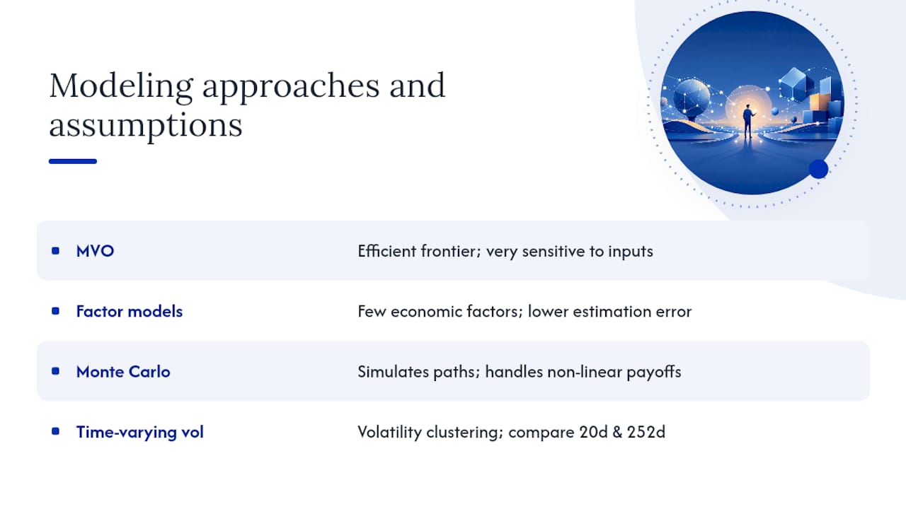
Modeling approaches and what each one assumes — overview diagram

Monte Carlo simulation generates thousands of possible return paths by sampling from a specified distribution (or from historical returns with replacement). It handles complex option payoffs, path-dependent strategies, and non-linear instruments that closed-form formulas cannot. The trade-off is computational cost and the risk of garbage-in-garbage-out: if your input distribution is wrong, your simulated tails are wrong too.

Time-varying volatility models like GARCH recognize that volatility clusters. A quiet market in January does not predict a quiet market in March. GARCH-family models estimate current volatility from recent squared returns and lagged variance, which produces risk estimates that respond to regime shifts. For individual investors, a practical shortcut is to monitor a 20-day realized volatility alongside your 252-day estimate and act when the gap widens materially.

Practitioners combine variance-based, tail, and contribution measures and validate with backtests and scenario tests — because no single risk measure is perfect for every market condition.

How to act on the analysis: practical risk-control strategies

Measuring risk without acting on it is just math homework. These four strategies translate numbers into portfolio decisions.

Set these limits before you need them, not after a position has already run up.

Diversification by factor, not just by count. Owning 30 stocks sounds diversified until you notice that 25 of them load heavily on the same growth factor. Tools like ETF.com’s overlap checker or a simple holdings export let you see the actual concentration before it shows up in your covariance matrix.

Threshold-based rebalancing. Calendar rebalancing (every quarter, no matter what) ignores the actual drift in your portfolio. This approach tends to reduce unnecessary turnover while catching real concentration events faster. For taxable accounts, combine the drift trigger with tax-lot awareness to minimize realized gains.

Hedging and insurance. Protective puts on a concentrated equity position, or a small allocation to an inverse ETF during high-volatility periods, can cap downside without requiring you to sell the underlying. These tools carry their own costs (option premium, tracking error) and are most appropriate when you have a specific, time-bounded risk you want to limit, not as a permanent portfolio feature. For most individual investors, cTrader risk management tools and similar real-time monitoring setups are worth exploring once you move from analysis to active management.

The answer often recalibrates what “acceptable risk” means faster than any formula will.*

Which tools actually help you run the analysis

The right tool depends on your portfolio size, technical comfort, and how often you need to repeat the analysis.

Tier 1: Spreadsheets (Excel or Google Sheets)

Best for portfolios under 20 positions and one-time or occasional analyses. Excel’s MMULT, TRANSPOSE, and COVARIANCE.S functions handle the core math. The main limitation is manual data entry and the ease of introducing formula errors that are hard to audit. Transparent and fast for small books; fragile at scale.

Tier 2: Python and R with open-source libraries

Python + pandas + NumPy: handles the full workflow described above, from return computation through VaR and CVaR.
Riskfolio-Lib: an open-source Python library that implements a broad set of portfolio optimization and risk measures, including CVaR, drawdown measures, and factor-based optimization. Well-documented and actively maintained.
R + PerformanceAnalytics: strong for time-series risk metrics and rolling-window analysis.

This tier suits investors comfortable with code who want full control over methodology and reproducibility.

Tier 3: No-code deterministic platforms

For investors who want institutional-grade analysis without writing code, platforms like Quantgenie translate strategy descriptions into deterministic algorithms, run reproducible backtests against validated market data, and surface portfolio risk metrics automatically. The key advantage over spreadsheets is auditability: every run produces the same output from the same inputs, which prevents the silent errors that plague manual workflows.

Data sources

Yahoo Finance (via yfinance in Python): free adjusted close data, good for most U.S. equities
FRED (Federal Reserve Economic Data): risk-free rates, macro series, and factor data
Broker historicals: most U.S. brokers (Schwab, Fidelity, Interactive Brokers) export transaction and price history directly
Limits of free data: survivorship bias (delisted stocks disappear), split-adjustment errors, and missing dividend adjustments are real problems for backtests longer than 5 years

Checklist for choosing a tool:

Does it produce reproducible results from the same inputs?
Can it aggregate across multiple accounts?
Does it generate automated alerts when risk thresholds are breached?
Is there an audit trail (data version + config + seed) for every run?

For prop trader performance improvement, the same checklist applies: reproducibility and real-time monitoring matter as much as the underlying math.

Graduate from spreadsheets when you have more than 20 positions, run the analysis more than monthly, or need to share results with anyone else who needs to verify them.

Why reproducible backtests matter more than most investors realize

A backtest that produces different results each time you run it is not a backtest. It is a random number generator with a narrative attached.

The CFA Institute’s risk management framework treats reproducibility and documented model governance as core professional standards, not optional extras. The practical reason is simple: if you cannot reproduce your risk estimate, you cannot tell whether a change in the number reflects a real change in portfolio risk or a change in your inputs, lookback window, or data source.

Reproducible pipelines catch look-ahead bias before it corrupts your conclusions. A non-reproducible workflow lets it hide indefinitely.

Here is a concrete failure mode. Suppose you backtest a momentum strategy and accidentally include the current month’s return in the signal calculation. The strategy looks exceptional in-sample. When you run it live, performance collapses. A deterministic pipeline with a fixed data snapshot and a logged config file would have flagged the date misalignment immediately. An ad-hoc spreadsheet would not.

Robustness checks to run on every analysis:

Rolling-window backtests: re-estimate risk metrics on a rolling 252-day window and check whether the estimates are stable or wildly variable across time.
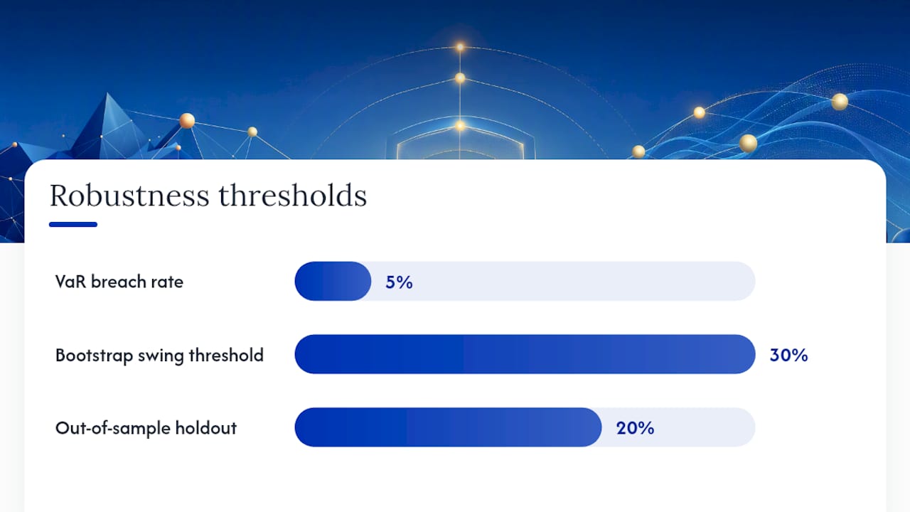
VaR exception rate: count how often actual losses exceed your VaR estimate. At 95% confidence, you should see breaches roughly 5% of trading days. Significantly more means your model underestimates risk; significantly fewer may mean it is too conservative.
Bootstrap sensitivity: resample your return history with replacement and recompute portfolio variance. If the estimate swings by more than 30% across bootstrap samples, your lookback window is too short.
Out-of-sample holdout: reserve the most recent 20% of your data as a holdout set. Never touch it during model development. Evaluate final risk estimates on the holdout only.

Pro Tip: Keep a minimal audit trail for every analysis: the exact data snapshot date, the config parameters (lookback, confidence level, rebalancing threshold), and a random seed if any simulation is involved. A plain text file works. Without it, you cannot reproduce your own conclusions six months later.

Why reproducible backtests matter more than most investors realize — overview diagram

Common pitfalls that break portfolio risk models

Most modeling failures are not exotic. They are the same four problems, repeated.

Estimation error in the covariance matrix. With 50 assets and 252 days of data, you are estimating 1,275 parameters from 12,600 observations. The sample covariance matrix is noisy. Ledoit-Wolf shrinkage (available in scikit-learn as LedoitWolf()) pulls extreme off-diagonal entries toward zero, producing a more stable estimate. Use it whenever your asset count is more than a fraction of your observation count.

Non-normal returns. Equity returns have fat tails and negative skew. The Cambridge text on portfolio theory addresses this directly: when returns deviate from normality, variance-based methods underestimate tail risk, and CVaR or scenario-based approaches produce more reliable controls. Check your return distribution with a QQ plot and compute skewness and excess kurtosis. If excess kurtosis exceeds 1.0, your parametric VaR is likely understating risk.

Backtest pathologies:

Look-ahead bias: using data that would not have been available at the decision point (e.g., end-of-day prices to generate intraday signals). Fix: timestamp every data point and enforce strict “as-of” data access.
Survivorship bias: backtesting only on stocks that still exist today. Fix: use a point-in-time universe that includes delisted securities.
Overfitting: tuning parameters until the backtest looks good, then treating in-sample results as predictive. Fix: set parameters before looking at results, use a holdout set, and apply a complexity penalty (fewer free parameters is better).
Data snooping: running hundreds of strategy variants and reporting the best one. Fix: pre-register your hypothesis before testing.

Model governance checklist:

Holdout window reserved before any parameter tuning
Out-of-sample test run exactly once on final model
Decision thresholds set conservatively (do not optimize the threshold itself)
VaR exception rate monitored monthly in live use
Model review scheduled at least annually or after any major market regime change

Reading your risk report and building an action plan

Numbers without a decision attached are just decoration. Here is how to turn a risk report into a short action plan you can implement this week.

Start with concentration and tail risk. Before looking at Sharpe ratios or alpha, check two things: which positions contribute the most to portfolio variance (risk contribution analysis), and what your CVaR looks like relative to your VaR.

Set two limits before you do anything else:

A position cap (e.g., no single stock above 5% of portfolio value)
A sector cap (e.g., no single sector above 25%)

These are not sophisticated. They are effective. Most individual investors who blow up do so because of concentration, not because they chose the wrong factor model.

Suggested initial policy:

Gather holdings and compute current weights
Run portfolio variance (w’ Σ w) and identify the top three risk contributors
Check CVaR at 95% confidence against your stated loss tolerance
Set position and sector caps based on what you find
Set a drift threshold for rebalancing (±5% from target weight is a reasonable starting point)
Schedule a monthly review of VaR exception rate and a quarterly full re-analysis

When to get professional help. Three red flags that suggest you should consult a registered investment advisor (verify credentials at Adviserinfo):

Your CVaR is more than twice your stated maximum tolerable loss
Your VaR model is breaching its confidence threshold more than twice the expected rate, and you cannot identify why
A single position or correlated cluster represents more than 30% of your total portfolio variance and you cannot reduce it without significant tax consequences

Immediate next steps (this week):

Export your holdings from your broker and compute current weights
Pull 2 years of adjusted close prices and compute annualized standard deviation for each position
Build the covariance matrix and compute w’ Σ w
Compare your portfolio CVaR to the maximum loss you could absorb without changing your financial plan

An analyst’s perspective on doing this work well

The biggest mistake individual investors make in risk analysis is treating it as a one-time event. They run the numbers once, feel reassured, and file the spreadsheet. Six months later, the portfolio has drifted, correlations have shifted, and the original analysis is describing a portfolio that no longer exists.

Cognitive biases make this worse. Anchoring to the volatility regime you first measured leads you to underweight the possibility that conditions have changed. Recency bias cuts the other way: after a volatile period, investors often over-hedge, locking in losses and missing the recovery. A simple countermeasure for both: set a calendar reminder to re-run your full analysis every quarter, regardless of how calm or chaotic markets feel. The discipline of regular re-estimation is more valuable than any single sophisticated model.

Start simple. A covariance matrix, portfolio variance, and a historical VaR are enough to make better decisions than most retail investors make. Validate your model against actual outcomes. Document your decisions and the reasoning behind them. The goal is not to predict the future; it is to understand your current exposure clearly enough to act on it deliberately.

Quantgenie makes portfolio risk analysis reproducible and code-free

Running a rigorous investment risk assessment manually is time-consuming, and the audit trail problem is real: most spreadsheet-based workflows cannot prove that last month’s analysis used the same data version and parameters as this month’s.

Quantgenie

Quantgenie solves that directly. The platform’s deterministic algorithm engine means every backtest run from the same inputs produces identical results, which is the foundation of trustworthy risk work. Describe your strategy in plain English, and Quantgenie translates it into a validated algorithm, runs it against institutional-grade market data, and surfaces portfolio risk metrics including drawdown, volatility, and performance attribution without requiring a single line of code. Multi-account aggregation, automated threshold alerts, and repeatable stress tests are built in, so the robustness checks described in this article are not manual tasks you have to remember. Direct broker integrations mean the gap between analysis and live trading is a decision, not a technical project.

If you want to run your first reproducible portfolio risk analysis without writing code, start on the Quantgenie platform or go straight to the no-code strategy builder to see how your strategy holds up against real market history.

Sources

These resources cover the full range from academic foundations to practical implementation.

This article is general information, not a substitute for advice from a qualified financial advisor. Consult a qualified financial professional about your own circumstances before acting on anything here.