Mean Reversion Strategies: Practical Recipes for Traders

Trader reviewing mean reversion charts at desk

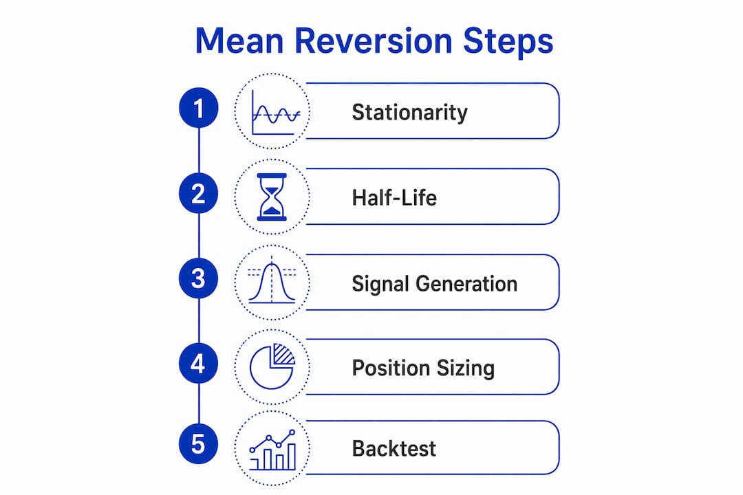
Mean reversion strategies exploit a simple but powerful idea: asset prices and spreads that drift away from a measurable historical average tend to return to it. The fastest path to applying this profitably is to confirm the series is stationary, measure how quickly it reverts, build a signal from z-scores or Bollinger Bands with an RSI confirmation, add an ADX regime filter to avoid trending markets, and backtest with realistic commissions and slippage before risking a dollar.

Before you trade any candidate instrument, run this quick validation:

Stationarity: ADF test p-value < 0.05, or Hurst exponent H < 0.5
Half-life: Compute ln(2)/θ from the Ornstein-Uhlenbeck fit; only trade if the half-life falls in a window you can hold
Signal: Enter when |z-score| > 2.0; exit at z = 0; hard stop at |z| > 3.5
Regime filter: ADX < 20 confirms a ranging market; skip the trade when ADX > 25
Cost check: Net Sharpe ratio after commissions and slippage must stay positive

The one rule that governs everything else: Only trade mean reversion when the series demonstrates statistical stationarity and your backtest remains profitable after including realistic slippage and commissions. Without that, you are gambling on noise.

Quantgenie’s no-code platform can run these exact validation steps and translate plain-English rules into deterministic algorithms, so the workflow below applies whether you code or not.

What mean reversion actually means for a trader
The statistical tests you need to run before anything else
Which indicators generate the clearest mean reversion signals
Three concrete mean reversion strategy examples you can backtest today
How to backtest and stress-test your strategy before going live
Risk controls and regime detection: when mean reversion fails
How to implement mean reversion without writing a single line of code
Choosing the right timeframe and lookback period for U.S. markets
Key Takeaways
The gap between what mean reversion promises and what actually survives contact with the market
Build and backtest your mean reversion strategy without writing code
Useful sources for going deeper

What mean reversion actually means for a trader

Mean reversion is the tendency of a price series or spread to oscillate around a stable long-run average rather than drift indefinitely in one direction. Statistically, this is called stationarity: the series has a constant mean and bounded variance over time. A random walk, by contrast, has no such anchor.

Analyst studying mean reversion stats overhead view

The workhorse model is the Ornstein-Uhlenbeck (OU) process, which describes how a value is pulled back toward its mean with a speed proportional to how far it has strayed. The key parameter is θ (the mean-reversion speed), and from it you derive the half-life: the expected time for the deviation to shrink by half, calculated as ln(2)/θ. A half-life of roughly 5 days implies active, short-term trading; a half-life of 60 or more days is usually too slow to trade profitably after costs.

Infographic showing mean reversion trading steps

Why does this matter practically? The half-life informs key trading parameters such as expected holding time, appropriate lookback periods for moving averages or z-scores, and trading frequency, which together influence total transaction costs.

Imagine a price chart where the series bounces repeatedly within a band around a moving average, touching the upper band and snapping back, touching the lower band and recovering. That visual is exactly what a mean-reverting spread looks like. Single-asset reversion does occur, but it is weaker and more regime-dependent than spread-based approaches.

Pro Tip: Prefer spread-based or ratio series (pairs trading) over single-asset mean reversion. A cointegrated pair creates a synthetic stationary series even when neither individual stock is stationary on its own, giving you a more reliable signal and a tighter statistical edge.

The statistical tests you need to run before anything else

Run four tests in sequence: the Augmented Dickey-Fuller (ADF) for stationarity, the Hurst exponent to classify process behavior, a cointegration test for pairs, and a half-life estimate to set your timeframe. Skip any of these and you are building on an untested foundation.

The four-test sequence

Augmented Dickey-Fuller (ADF) test. Feed the price series (or spread) into the ADF. The null hypothesis is a unit root (non-stationary). You want to reject it: a p-value below 0.05 means the series is stationary at the 5% confidence level. Use at least 252 trading days of data for a reliable result.
Hurst exponent (H). H < 0.5 indicates mean-reverting behavior; H = 0.5 is a random walk; H > 0.5 is trending. Compute it using rescaled-range analysis or a variance-ratio method. Think of it as a second opinion on the ADF result.
Cointegration test (pairs only). For two-asset spreads, run the Engle-Granger two-step test or the Johansen test. Engle-Granger regresses one asset on the other and then runs ADF on the residuals. Johansen handles multiple assets and is more robust when the hedge ratio is uncertain.
Half-life estimation. Regress the daily change in the spread on its lagged level: ΔS(t) = a + b·S(t-1) + ε. The half-life is ln(2) / |b|. This number sets your lookback window and expected holding period.

Interpretation table

Test result	Meaning	Trading action
ADF p < 0.05	Series is stationary	Proceed to half-life and signal design
ADF p > 0.10	Series is non-stationary	Reject; do not trade mean reversion
H < 0.5	Mean-reverting process	Confirms ADF; proceed
H > 0.5	Trending process	Reject or switch to momentum
Cointegration confirmed	Spread is stationary	Build pairs strategy on this spread
Half-life < 2 days	Too fast for most retail execution	Avoid unless you have low-latency infrastructure
Half-life > 60 days	Too slow; cost drag likely fatal	Avoid or use very wide stops

Pseudocode: the validation sequence

1. Load price series (or construct spread = P1 - hedge_ratio * P2)
2. Run ADF(series) → if p_value > 0.05: STOP
3. Compute Hurst(series) → if H >= 0.5: flag warning
4. Regress delta_S on lagged_S → extract b → half_life = ln(2) / abs(b)
5. If half_life < 2 or half_life > 60: STOP (adjust thresholds to your execution)
6. Set lookback = round(half_life * 2)
7. Proceed to signal construction

One practical caveat: markets change. Run a rolling ADF over a 252-day window and check for structural breaks using a Chow test or CUSUM method. A spread that was cointegrated for two years can break down after a merger, earnings surprise, or macro regime shift. Catching that early saves significant drawdown.

Which indicators generate the clearest mean reversion signals

The three workhorses are the z-score of a spread, Bollinger Bands, and RSI(2). Each measures deviation from a mean differently; combining two of them for confirmation reduces false signals without requiring a complex model.

Indicator thresholds

Indicator	Setting	Entry signal	Exit signal	Stop
Z-score (spread)	Lookback = half-life × 2		z	> 2.0
Bollinger Bands	20-period SMA, ±2σ	Price touches lower/upper band	Price crosses SMA	Close outside band for 3+ bars
RSI(2)	2-period RSI	RSI < 10 (long) / > 90 (short)	RSI > 40 (long exit) / < 60 (short exit)	Hard price stop
ADX (regime filter)	14-period	ADX < 20: trade allowed	N/A	ADX > 25: exit or pause

Example rule sets

Single-asset intraday (Bollinger + RSI(2)):

Long entry: price closes below lower Bollinger Band AND RSI(2) < 10
Exit: price crosses the 20-period SMA OR RSI(2) > 40
Stop: close below the band for three consecutive bars (structural break signal)

Pairs spread (z-score):

Long spread: z-score < -2.0 (spread is abnormally low)
Short spread: z-score > 2.0 (spread is abnormally high)
Exit both legs: z-score crosses zero
Hard stop: |z| > 3.5 to limit losses from structural breaks

Pro Tip: Always pair a volatility-normalized signal like the z-score with an ADX regime filter. A z-score of 2.5 in a trending market is not a reversion opportunity — it is a continuation setup in disguise. The ADX gate keeps you out of those traps.

Timeframe matters here. A short half-life (5–10 days) supports intraday or daily RSI(2) signals. A longer half-life (20–40 days) needs wider Bollinger Bands and a slower moving average, or the signal fires too early and you sit through a deeper drawdown before the reversion arrives.

Three concrete mean reversion strategy examples you can backtest today

1. Pairs trading recipe (equities)

Two traders discussing pairs trading strategy

Pairs trading is the most statistically reliable mean-reversion approach in equities because you construct a spread that is stationary by design.

Step-by-step:

Screen for candidate pairs with high historical correlation (r > 0.80 over 252 days)
Run Engle-Granger cointegration on each candidate; keep only pairs with p < 0.05
Estimate the hedge ratio β from the regression: P1 = α + β·P2
Construct the spread: S = P1 - β·P2
Compute the rolling z-score of S using a lookback equal to twice the half-life
Enter long spread when z < -2.0; enter short spread when z > 2.0
Exit when z returns to 0; stop at |z| > 3.5

Numeric example: Stock A trades at $50, Stock B at $25, hedge ratio β = 2.0. Spread = $50 - 2.0 × $25 = $0. If Stock A drops to $46 while Stock B holds at $25, spread = $46 - $50 = -$4. If the historical spread standard deviation is $2, z = -4/2 = -2.0. That triggers a long entry: buy Stock A, short Stock B. When the spread returns to $0, close both legs.

Position sizing: Size each leg so that a 1-standard-deviation move in the spread equals 1% of portfolio equity. This keeps exposure proportional to the signal’s statistical uncertainty.

2. Intraday mean reversion recipe (single asset)

This approach works on liquid U.S. equities or ETFs with tight bid-ask spreads. The half-life here is typically 1–3 days.

Checklist before trading:

Confirm ADF p < 0.05 on a 60-day rolling window
ADX(14) < 20 at the time of signal
Spread between bid and ask is less than 0.05% of price

Entry/exit rules:

Long: price closes below lower Bollinger Band (20, 2σ) AND RSI(2) < 10
Exit long: price crosses 20-period SMA OR RSI(2) > 40
Short: price closes above upper band AND RSI(2) > 90
Exit short: price crosses 20-period SMA OR RSI(2) < 60
Hard stop: 2× the average true range from entry

Expected hold time aligns with a short half-life consistent with intraday or short-term trading.

3. FX mean reversion notes

Mean reversion can work on major FX pairs (EUR/USD, USD/JPY) during range-bound macro environments, but the half-lives tend to be longer and the regime shifts more abrupt. Use wider z-score thresholds (entry at |z| > 2.5, stop at |z| > 4.0) and a longer lookback (60–90 days). Watch for central bank announcements and macro data releases, which can trigger structural breaks that invalidate the stationarity assumption overnight. FX mean reversion is best treated as a secondary strategy with smaller position sizes relative to your equity pairs book.

How to backtest and stress-test your strategy before going live

A backtest that ignores transaction costs is not a backtest. It is a fantasy. Mean reversion strategies trade frequently, and their per-trade edge is narrow, so costs can easily consume the entire alpha.

Backtest checklist

Data quality: Use adjusted prices; remove survivorship bias by including delisted securities
Lookahead bias: Never use today’s close to generate today’s signal; signals must use only data available at the time of the trade
Transaction cost model: Include commissions (per share or per trade) and a slippage estimate (typically 0.01%–0.05% per side for liquid U.S. equities)
Realistic fills: Assume limit orders may not fill; model partial fills for larger positions
Walk-forward validation: Split data into in-sample (training) and out-of-sample (test) periods; repeat across rolling windows
Structural break check: Test performance before and after major market events (2008, 2020)

Performance metrics to report

Metric	What it measures	Minimum threshold to consider live
Net CAGR	Annualized return after all costs	Positive and meaningful vs. benchmark
Sharpe ratio (net)	Risk-adjusted return	> 0 after costs
Max drawdown	Worst peak-to-trough loss	< 20% for most retail traders
Win rate	% of profitable trades	> 50% for mean reversion
Average trade (net)	Mean P&L per trade after costs	Must be positive
Expectancy	Win rate × avg win - loss rate × avg loss	Must be positive
Transaction cost burden	Total costs as % of gross profit	< 30% is a reasonable ceiling

Pro Tip: Integrate your commission and slippage model from the very first backtest run, not as an afterthought. High-turnover mean reversion strategies are especially sensitive to costs — a strategy showing a 1.5 Sharpe gross can drop below 0.5 net once realistic fills are modeled.

Robustness checks go beyond a single in-sample/out-of-sample split. Run a walk-forward validation with at least five rolling windows. Build a parameter sensitivity heatmap: vary your z-score entry threshold from 1.5 to 3.0 and your lookback from half the half-life to twice it. If performance collapses when you nudge a parameter by 10%, the strategy is overfit. Bootstrap resampling of trade returns gives you a distribution of Sharpe ratios rather than a single point estimate, which is far more honest about what you can expect.

Risk controls and regime detection: when mean reversion fails

Mean reversion fails in trending markets. That is not a caveat; it is the primary failure mode. ADX below 20 signals a ranging market where mean reversion tends to work; ADX above 25 signals a trending market where it reliably causes drawdowns.

Risk control checklist

Hard stop: Exit any position when |z| > 3.5; this limits losses from structural breaks where the spread never reverts
Time stop: Close any position that has not reverted within 2× the half-life; holding longer usually means the assumption has broken down
Portfolio exposure cap: Limit total mean-reversion exposure to a fixed percentage of portfolio equity (many practitioners use 20%–30%)
Diversification: Run multiple uncorrelated spreads; a single spread that breaks can be catastrophic if it represents your entire book
ADX gate: Check ADX before every new entry; skip the trade if ADX > 25

Position sizing

A simple volatility-parity approach works well: size each trade so that the expected dollar volatility of the position equals a fixed fraction of portfolio equity. For example, if your target risk per trade is 0.5% of equity and the spread has a daily standard deviation of $2, your position size is (0.005 × equity) / $2. Apply a Kelly fraction cap (never exceed half-Kelly) to avoid ruin from model error.

Shorter half-lives allow more frequent trades but require smaller individual sizes because the cumulative cost burden grows with turnover. Longer half-lives support larger positions but demand wider stops and more capital tied up per trade.

Regulatory note: Ensure your order types, margin usage, and position limits conform to your U.S. broker’s rules and FINRA/SEC requirements before deploying any live strategy.

How to implement mean reversion without writing a single line of code

You do not need Python to run a rigorous mean-reversion workflow. The full sequence from stationarity testing to live deployment can be executed on a no-code platform that translates plain-English rules into deterministic algorithms.

No-code workflow steps

Define the instrument: Select your asset or pair from the platform’s data library; choose the date range covering at least 252 trading days
Run stationarity tests: Use the built-in ADF and Hurst modules; set the significance threshold and review the output before proceeding
Estimate half-life: Use the platform’s OU parameter estimator; let the result auto-populate your lookback period
Build the signal: Select z-score, Bollinger Bands, or RSI(2) from the signal library; enter your thresholds (entry, exit, stop) in plain English or via a visual editor
Add the regime filter: Drop in an ADX module; set the gate at ADX < 20 for entries
Configure the cost model: Enter your broker’s commission rate and a slippage estimate; the platform applies these to every simulated fill
Run walk-forward backtest: Set in-sample and out-of-sample windows; review the robustness heatmap and rolling Sharpe chart
Inspect and refine: Use AI-assisted Q&A on backtest results to identify weak parameters before touching live capital

Step-by-step on Quantgenie

Log in and create a new strategy
Describe your mean-reversion logic in plain English (e.g., “Buy when the 20-day z-score of the spread falls below -2; exit when z returns to 0; stop if |z| exceeds 3.5”)
Quantgenie translates this into a deterministic algorithm with no ambiguity
Select institutional-grade historical data for your target instruments
Run the ADF and Hurst validation modules; review pass/fail before proceeding
Configure the ADX regime filter and transaction cost model
Execute walk-forward backtesting; review the Sharpe, drawdown, and cost-burden metrics
Deploy to your broker via direct integration when the strategy passes all checks

The key advantage of a no-code platform like Quantgenie is determinism: the same plain-English rule produces the same algorithm every time, which means your backtest results are reproducible and your live execution matches what you tested.

Choosing the right timeframe and lookback period for U.S. markets

Timeframe selection is not arbitrary. It flows directly from the half-life of the series you are trading, and U.S. market microstructure adds a few additional constraints worth knowing.

Daily timeframe (most common for retail traders): Works well for pairs with half-lives of 5–20 days. Use a lookback of roughly twice the half-life for your z-score or Bollinger Band calculation. Most U.S. equity pairs and sector ETF spreads fall in this range. The daily close is a clean, well-defined price point that avoids intraday noise and reduces the impact of bid-ask spread on signal quality.

Intraday (60-minute or 15-minute bars): Suitable for half-lives of 1–3 days when measured on daily data, which often translates to 8–24 intraday bars. U.S. equity markets open with a volatility burst in the first 30 minutes; many intraday mean-reversion traders avoid signals generated in that window and focus on the 10:00 AM to 3:30 PM ET session. Costs matter more here because you trade more frequently.

Weekly timeframe: Appropriate for spreads with half-lives of 20–60 days. Sector rotation pairs and commodity spreads sometimes fall here. The lookback for a weekly z-score might be 10–20 weeks. Transaction costs are lower per trade, but capital is tied up longer and you need wider stops to accommodate normal weekly volatility.

Lookback calibration for U.S. equities: A practical starting point is to run the ADF and half-life estimation on at least two years of daily data (roughly 504 trading days). This captures at least one full market cycle and gives the cointegration test enough power to be meaningful. Avoid using more than five years without a structural-break check, since company fundamentals and sector compositions shift over that horizon.

One U.S.-specific consideration: earnings seasons (January, April, July, October) and Federal Reserve announcement dates can temporarily break mean-reverting relationships. Many practitioners pause new entries in the 48 hours surrounding major macro events and resume once volatility normalizes. This is not a formal rule but a practical habit that protects against the most predictable structural disruptions.

Key Takeaways

Mean reversion strategies only work when the underlying series is statistically stationary — validate that first, measure the half-life second, and never skip the cost model in your backtest.

Point	Details
Validate stationarity first	Run ADF (p < 0.05) and Hurst (H < 0.5) before building any signal or backtest.
Half-life drives everything	Compute ln(2)/θ to set your lookback, expected hold time, and position size.
Use z-scores with a regime filter	Enter at
Costs can kill a valid strategy	Include commissions and slippage from the first backtest run; net Sharpe must stay positive.
Quantgenie removes the coding barrier	Translate plain-English mean-reversion rules into deterministic algorithms and run walk-forward backtests without writing code.

The gap between what mean reversion promises and what actually survives contact with the market

Most traders who blow up on mean reversion strategies do not fail because the math is wrong. They fail because they skip the regime filter, underestimate transaction costs, or hold a broken spread hoping it will revert. The statistical edge is real, but it is narrow, and it disappears fast when conditions change.

The practical lesson I keep coming back to: half-life is the most underused number in mean reversion. Traders spend hours tuning z-score thresholds and almost no time on the half-life estimate, yet half-life governs how long you hold, how often you trade, and therefore how much you pay in costs. A strategy with a 3-day half-life and a 0.10% round-trip cost burden is a very different animal from one with a 15-day half-life and the same cost structure. The first one needs near-zero commissions to survive; the second has room to breathe.

The other thing that rarely gets said plainly: pairs trading is not passive. The cointegration relationship between two stocks can break permanently after a merger, a credit event, or a major product cycle shift. Running a rolling ADF every 20 trading days and being willing to close a pair that no longer passes is not optional maintenance. It is the core risk management act of the strategy. Traders who treat the initial cointegration test as a one-time credential and then hold the spread for months are the ones who end up with the horror stories.

Position sizing tied to volatility parity, a hard stop at |z| > 3.5, and a time stop at 2× the half-life are not conservative choices. They are the minimum viable risk controls for a strategy that, by design, bets against the current price move. The market is not always wrong when it trends.

Build and backtest your mean reversion strategy without writing code

Most traders who understand the math still get stuck at implementation. Writing Python to run ADF tests, construct spreads, apply regime filters, and model transaction costs takes weeks to build and months to trust. Quantgenie cuts that path to hours.

Quantgenie

Describe your mean-reversion logic in plain English and Quantgenie translates it into a deterministic algorithm with no ambiguity between what you intended and what gets tested. The platform includes built-in ADF and Hurst validation modules, half-life calculators, z-score and Bollinger Band signal builders, ADX regime filters, and a walk-forward backtesting engine that applies your actual commission and slippage assumptions to every simulated fill. Every backtest run produces identical results under the same conditions, so you are comparing apples to apples when you iterate on parameters.

The performance dashboard surfaces net CAGR, Sharpe ratio, max drawdown, and transaction cost burden in one view, and the AI-assisted Q&A feature lets you interrogate your backtest results without needing to write a single query. When the strategy passes your robustness checks, direct broker integrations handle live deployment.

Start your first mean-reversion backtest on Quantgenie today and see whether your candidate instruments pass the stationarity tests before you risk any capital.

Useful sources for going deeper

The sources below back the key claims in this article and are worth bookmarking for code examples, mathematical derivations, and conceptual depth.

Basics of Statistical Mean Reversion Testing — QuantStart. The clearest explanation of ADF, Hurst exponent, and half-life estimation available for practitioners. Start here for the math and Python pseudocode behind the tests described in this article.
Mean Reversion (Finance) — Wikipedia). A solid conceptual overview covering the theory, asset classes where mean reversion appears, and links to related strategies including pairs trading and statistical arbitrage.
Ornstein-Uhlenbeck Process — Wikipedia. The mathematical foundation for the OU model and half-life formula. Useful if you want to understand the stochastic differential equation behind the intuition.
statsmodels ADF documentation. The reference for running the Augmented Dickey-Fuller test in Python. Covers parameters, output interpretation, and regression options.
Mean Reversion Strategies — QuantifiedStrategies. Backtested rule sets with performance data across U.S. equities. Good for benchmarking your own results against published strategies.
Mean Reversion Strategies: Introduction — Interactive Brokers Campus. Covers implementation in a brokerage context, including order types and practical execution considerations relevant to U.S. retail traders.
Mean Reversion Trading Strategy — QuantVero. Detailed walkthrough of walk-forward validation, sensitivity heatmaps, and bootstrap resampling for robustness testing.

For U.S.-specific broker rules, margin requirements, and order type restrictions, consult your broker’s documentation directly and review FINRA’s published guidelines. Regulatory requirements change; always verify current rules before deploying a live strategy.

This article is general educational information, not financial or investment advice. Confirm current regulations and suitability with a qualified financial professional before trading.